Overview
Running ERFs on a given dataset is easy. The function ens_random_forests() will take a given dataset in R data.frame format, amend it for modeling using erf_data_prep() and erf_formula_prep(), run each RF in the ensemble using rf_ens_fn(), and return a fitted ERF object. This object can then be passed to various output functions: erf_plotter() and … to visualize and summarize.
First, we must load the R library.
library(EnsembleRandomForests)
#> Loading required package: doParallel
#> Loading required package: foreach
#> Loading required package: iterators
#> Loading required package: parallel
#> Loading required package: randomForest
#> randomForest 4.7-1.1
#> Type rfNews() to see new features/changes/bug fixes.
Datasets
Using the provided simulated dataset
The provided dataset is a list object that contains a data.frame of the sampled locations, the beta coefficients of the logistic model used to predict the probability of occurrence, and a raster brick object containing the gridded covariates, log-odds of occurrence, and probabilities of occurrence.
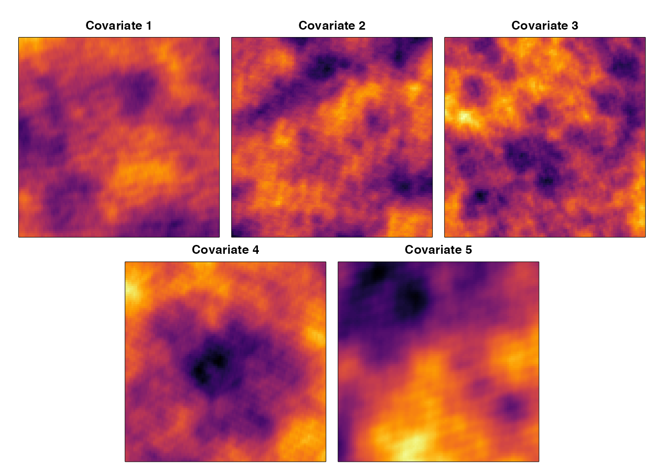
# We can also visualize the covariates
par(mar=c(0,0.5,2,0.5), oma=c(1,1,1,1))
layout(matrix(c(1,1,2,2,3,3,0,4,4,5,5,0),2,6,byrow=TRUE))
r <- range(cellStats(simData$grid[[1:5]],'range'))
for(i in 1:5){
  image(simData$grid[[i]], col=inferno(100), zlim = r,
        xaxt='n', yaxt='n', xlab="", ylab="")
  title(paste0('Covariate ', i))
}
We can also see the beta coefficients that produced the probability of presence using the model below: \[\begin{equation} log\left[\frac{\hat{P}_{obs=1}}{1-\hat{P}_{obs=1}}\right] = \alpha + \beta_1X_1 + ... +\beta_nX_n \end{equation}\]
print(round(simData$betas,3))
#> [1] -8.683 -2.642 -2.400  7.535  2.148

# We can visualize the log-odds and the probability of presence
par(mar=c(0,0.5,2,0.5), oma=c(1,1,1,1), mfrow=c(1,2))
image(simData$grid[[6]], col=inferno(100), xaxt='n', yaxt='n', xlab="", ylab="")
title("Log-odds")
image(simData$grid[[7]], col=viridis(100), xaxt='n', yaxt='n', xlab="", ylab="")
with(simData$samples[simData$samples$obs==1,],
     points(x,y,pch=16,col='white'))
title("Probability of Presence")
Running an Ensemble Random Forests model
Now that we have covered the datasets, let’s run an ERF. This is simple using ens_random_forests.
ens_rf_ex <- ens_random_forests(df=simData$samples, var="obs",
                                covariates=grep("cov",colnames(simData$samples),value=T),
                                header = NULL,
                                save=FALSE,
                                out.folder=NULL,
                                duplicate = TRUE,
                                n.forests = 10L,
                                importance = TRUE,
                                ntree = 1000,
                                mtry = 5,
                                var.q = c(0.1,0.5,0.9),
                                cores = parallel::detectCores()-2)
#> rounding n.forests to the nearest one
The arguments to ens_random_forests are:
- Data arguments:
-
df: this is the data.frame containing the presences/absences and the covariates -
var: this is the column name of the presence/absence -
covariates: these are the column names of the covariates to use. Here, we grabbed anything with “cov” in the column name -
header: these are additional column names you may wish to append to data.frame produced internally
-
- Output arguments:
-
save: this is a logical whether to save the model to the working directory or an optionalout.folderdirectory
-
- Control arguments:
-
duplicate: a logical flag to control whether to duplicate observations with more than one presence. -
n.forests: this controls the number of forests to generate in the ensemble. See the optimization vignette for more information on tuning this parameter. -
importance: a logical flag to calculate variable importance or not -
ntree: number of trees in each Random Forests in the ensemble -
mtry: number of covariates to try at each node in each tree in each Random Forests in the ensemble -
var.q: quantiles for the distribution of the variable importance; only exectuted if importance=TRUE -
cores: how many cores to run the model on.
-
We can look at some of the output produced by the random forests (see help(ens_random_forests) for a full list):
#view the dataset used in the model
head(ens_rf_ex$data)
#>   obs        cov1        cov2       cov3        cov4        cov5     random
#> 1   0 -0.07158000 -0.27811766  0.5741324  0.01366734 -0.15537696  1.9850664
#> 2   0 -0.12028137  0.26103341 -0.2298234  0.14750795  0.32482174  0.4330434
#> 3   0  0.12422049  0.09052045 -0.3070963  0.14493653  0.02303010 -0.1619807
#> 4   0 -0.12481261 -0.29583389  0.6282519  0.06067430 -0.25240678  0.9201079
#> 5   0  0.01361460 -0.04989738  0.1600218  0.42189437  0.13166581  1.1538205
#> 6   0  0.01842766  0.18300638 -0.3421439 -0.33128857  0.07998399 -1.4189254

#view the ensemble model predictions
head(ens_rf_ex$ens.pred)
#>      P.0    P.1 PRES   resid
#> 1 0.7339 0.2661    0 -0.2661
#> 2 0.3457 0.6543    0 -0.6543
#> 3 0.5991 0.4009    0 -0.4009
#> 4 0.7706 0.2294    0 -0.2294
#> 5 0.3435 0.6565    0 -0.6565
#> 6 0.9928 0.0072    0 -0.0072

#view the threshold-free ensemble performance metrics
unlist(ens_rf_ex$ens.perf[c('auc','rmse','tss')])
#>       auc      rmse       tss
#> 0.9750790 0.3789975 0.8266660

#view the mean test threshold-free performance metrics for each RF
ens_rf_ex$mu.te.perf
#>     teAUC    teRMSE     teTSS
#> 0.7784570 0.3903881 0.5420088

#structure of the individual model predictions
str(ens_rf_ex$pred)
#> List of 2
#>  $ p    : num [1:10000, 1:10] 0.25 0.64 0.423 0.245 0.639 0.008 0.004 0.669 0.01 0.668 ...
#>  $ resid: num [1:10000, 1:10] -0.25 -0.64 -0.423 -0.245 -0.639 -0.008 -0.004 -0.669 -0.01 -0.668 ...
As we can see, the ensemble performs better than the mean test predictions. This is advantage of ERF over other RF modifications for extreme class imbalance. Siders et al. 2020 discusses the various performance of these other modifications if you are curious.